Table Of Content
Share this article:


Extract real-time Quick Commerce & FMCG data to boost pricing, trends, and sales insights.
Extract accurate Vacation Rental data with ease to track pricing, listings, and trends.
Get detailed Restaurant data like menus, ratings, and contacts with powerful extraction.
Efficiently extract Event and Meeting data for streamlined planning and insights.
AI-driven web scraping for accurate, automated data extraction—saving time & boosting insights.
Extract data tailored to your unique business needs with custom solutions.
Scrape data from mobile apps for detailed insights and competitor analysis.
Access structured web data effortlessly using our smart Web Scraping API solution.
Develop scalable web crawlers for fast, automated, and efficient data collection.
Extract real-time data from dynamic websites for timely insights and market advantage.
Track competitor pricing trends and stay ahead with smart Price Monitoring Services.
Track and analyze your brand's online presence to enhance reputation and drive growth.
Accurately match identical products across platforms to boost sales and visibility.
Transform your data into insightful visuals for better decision-making and analysis.
Extract and analyze online data with powerful Web Data Mining for smarter decisions and competitive growth.
Understand customer opinions and feedback with accurate Sentiment Analysis solution.
Monitor product visibility, pricing, and performance across online stores with advanced Digital Shelf Analytics solutions.
Boost data accuracy and efficiency with machine learning-based web scraping for smart automation.
High-quality AI training datasets for accurate models, automation, and smarter insights.
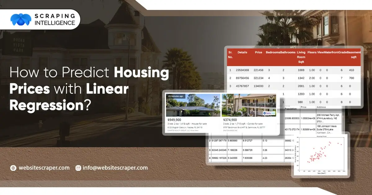
The final objective is to estimate the cost of a certain house in a Boston suburb. In 1970, the Boston Standard Metropolitan Statistical Area provided the information. To examine and modify the data, we will use several techniques such as data pre-processing and feature engineering. After that, we'll apply a statistical model like regression model to anticipate and monitor the real estate market.
Project Outline:
Before using a statistical model, the EDA is a good step to go through in order to:
# Import the libraries

#Dataframe/Numerical libraries
import pandas as pd
import numpy as np

#Data visualization
import plotly.express as px
import matplotlib
import matplotlib.pyplot as plt
import seaborn as sns

#Machine learning model
from sklearn.linear_model import LinearRegression
#Reading the data
path='./housing.csv'
housing_df=pd.read_csv(path,header=None,delim_whitespace=True)
| CRIM | ZN | INDUS | CHAS | NOX | RM | AGE | DIS | RAD | TAX | PTRATIO | B | LSTAT | MEDV | |
|---|---|---|---|---|---|---|---|---|---|---|---|---|---|---|
| 0 | 0.00632 | 18.0 | 2.31 | 0 | 0.538 | 6.575 | 65.2 | 4.0900 | 1 | 296.0 | 15.3 | 396.90 | 4.98 | 24.0 |
| 1 | 0.02731 | 0.0 | 7.07 | 0 | 0.469 | 6.421 | 78.9 | 4.9671 | 2 | 242.0 | 17.8 | 396.90 | 9.14 | 21.6 |
| 2 | 0.02729 | 0.0 | 7.07 | 0 | 0.469 | 7.185 | 61.1 | 4.9671 | 2 | 242.0 | 17.8 | 392.83 | 4.03 | 34.7 |
| 3 | 0.03237 | 0.0 | 2.18 | 0 | 0.458 | 6.998 | 45.8 | 6.0622 | 3 | 222.0 | 18.7 | 394.63 | 2.94 | 33.4 |
| 4 | 0.06905 | 0.0 | 2.18 | 0 | 0.458 | 7.147 | 54.2 | 6.0622 | 3 | 222.0 | 18.7 | 396.90 | 5.33 | 36.2 |
| ... | ... | ... | ... | ... | ... | ... | ... | ... | ... | ... | ... | ... | ... | ... |
| 501 | 0.06263 | 0.0 | 11.93 | 0 | 0.573 | 6.593 | 69.1 | 2.4786 | 1 | 273.0 | 21.0 | 391.99 | 9.67 | 22.4 |
| 502 | 0.04527 | 0.0 | 11.93 | 0 | 0.573 | 6.120 | 76.7 | 2.2875 | 1 | 273.0 | 21.0 | 396.90 | 9.08 | 20.6 |
| 503 | 0.06076 | 0.0 | 11.93 | 0 | 0.573 | 6.976 | 91.0 | 2.1675 | 1 | 273.0 | 21.0 | 396.90 | 5.64 | 23.9 |
| 504 | 0.10959 | 0.0 | 11.93 | 0 | 0.573 | 6.794 | 89.3 | 2.3889 | 1 | 273.0 | 21.0 | 393.45 | 6.48 | 22.0 |
| 505 | 0.04741 | 0.0 | 11.93 | 0 | 0.573 | 6.030 | 80.8 | 2.5050 | 1 | 273.0 | 21.0 | 396.90 | 7.88 | 11.9 |
Crime: It refers to a town's per capita crime rate.
ZN: It is the percentage of residential land allocated for 25,000 square feet.
Indus: The amount of non-retail business lands per town is referred to as the indus.
CHAS: CHAS denotes whether or not the land is surrounded by a river.
NOX: The NOX stands for nitric oxide content (part per 10m).
RM: The average number of rooms per home is referred to as RM.
AGE: The percentage of owner-occupied housing built before 1940 is referred to as AGE.
DIS: Weighted distance to five Boston employment centers are referred to as dis.
RAD: Accessibility to radial highways index.
TAX: The TAX columns denote the rate of full-value property taxes per $10,000 dollars.
B: B=1000(Bk — 0.63)² is the outcome of the equation, where Bk is the proportion of blacks in each town.
PTRATIO: It refers to the student-to-teacher ratio in each community.
LSTAT: It refers to the population's lower socioeconomic status.
MEDV: It refers to the 1000-dollar median value of owner-occupied residences.
# Check if there is any missing values.
housing_df.isna().sum()

CRIM       0
ZN         0
INDUS      0
CHAS       0
NOX        0
RM         0
AGE        0
DIS        0
RAD        0
TAX        0
PTRATIO    0
B          0
LSTAT      0
MEDV       0
dtype: int64
No missing values are found
We examine our data's mean, standard deviation, and percentiles.
housing_df.describe()
| CRIM | ZN | INDUS | CHAS | NOX | RM | AGE | DIS | RAD | TAX | PTRATIO | B | LSTAT | MEDV | |
|---|---|---|---|---|---|---|---|---|---|---|---|---|---|---|
| count | 506.000000 | 506.000000 | 506.000000 | 506.000000 | 506.000000 | 506.000000 | 506.000000 | 506.000000 | 506.000000 | 506.000000 | 506.000000 | 506.000000 | 506.000000 | 506.000000 |
| mean | 3.613524 | 11.363636 | 11.136779 | 0.069170 | 0.554695 | 6.284634 | 68.574901 | 3.795043 | 9.549407 | 408.237154 | 18.455534 | 356.674032 | 12.653063 | 22.532806 |
| std | 8.601545 | 23.322453 | 6.860353 | 0.253994 | 0.115878 | 0.702617 | 28.148861 | 2.105710 | 8.707259 | 168.537116 | 2.164946 | 91.294864 | 7.141062 | 9.197104 |
| min | 0.006320 | 0.000000 | 0.460000 | 0.000000 | 0.385000 | 3.561000 | 2.900000 | 1.129600 | 1.000000 | 187.000000 | 12.600000 | 0.320000 | 1.730000 | 5.000000 |
| 25% | 0.082045 | 0.000000 | 5.190000 | 0.000000 | 0.449000 | 5.885500 | 45.025000 | 2.100175 | 4.000000 | 279.000000 | 17.400000 | 375.377500 | 6.950000 | 17.025000 |
| 50% | 0.256510 | 0.000000 | 9.690000 | 0.000000 | 0.538000 | 6.208500 | 77.500000 | 3.207450 | 5.000000 | 330.000000 | 19.050000 | 391.440000 | 11.360000 | 21.200000 |
| 75% | 3.677083 | 12.500000 | 18.100000 | 0.000000 | 0.624000 | 6.623500 | 94.075000 | 5.188425 | 24.000000 | 666.000000 | 20.200000 | 396.225000 | 16.955000 | 25.000000 |
| max | 88.976200 | 100.000000 | 27.740000 | 1.000000 | 0.871000 | 8.780000 | 100.000000 | 12.126500 | 24.000000 | 711.000000 | 22.000000 | 396.900000 | 37.970000 | 50.000000 |
The crime, area, sector, nitric oxides, 'B' appear to have multiple outliers at first look because the minimum and maximum values are so far apart. In the Age columns, the mean and the Q2(50 percentile) do not match.
We might double-check it by examining the distribution of each column.
Because the model is overly generic, removing all outliers will underfit it. Keeping all outliers causes the model to overfit and become excessively accurate. The data's noise will be learned.
The approach is to establish a happy medium that prevents the model from becoming overly precise. When faced with a new set of data, however, they generalise well.
We'll keep numbers below 600 because there's a huge anomaly in the TAX column around 600.
new_df=housing_df[housing_df['TAX']<600]
The overall distribution, particularly the TAX, PTRATIO, and RAD, has improved slightly.
Perfect correlation is denoted by the clear values. The medium correlation between the columns is represented by the reds, while the negative correlation is represented by the black.
With a value of 0.89, we can see that 'MEDV', which is the medium price we wish to anticipate, is substantially connected with the number of rooms 'RM'. The proportion of black people in area 'B' with a value of 0.19 is followed by the residential land 'ZN' with a value of 0.32 and the percentage of black people in area 'ZN' with a value of 0.32.
The metrics that are most connected with price will be plotted.
Gradient descent is aided by feature scaling, which ensures that all features are on the same scale. It makes locating the local optimum much easier.
Mean standardization is one strategy to employ. It substitutes (target-mean) for the target to ensure that the feature has a mean of nearly zero.
def standard(X):
    '''Standard makes the feature 'X' have a zero mean'''
    mu=np.mean(X) #mean
    std=np.std(X) #standard deviation
    sta=(X-mu)/std # mean normalization
    return mu,std,sta

mu,std,sta=standard(X)
X=sta
X
| CRIM | ZN | INDUS | CHAS | NOX | RM | AGE | DIS | RAD | TAX | PTRATIO | B | LSTAT | |
|---|---|---|---|---|---|---|---|---|---|---|---|---|---|
| 0 | -0.609129 | 0.092792 | -1.019125 | -0.280976 | 0.258670 | 0.279135 | 0.162095 | -0.167660 | -2.105767 | -0.235130 | -1.136863 | 0.401318 | -0.933659 |
| 1 | -0.575698 | -0.598153 | -0.225291 | -0.280976 | -0.423795 | 0.049252 | 0.648266 | 0.250975 | -1.496334 | -1.032339 | -0.004175 | 0.401318 | -0.219350 |
| 2 | -0.575730 | -0.598153 | -0.225291 | -0.280976 | -0.423795 | 1.189708 | 0.016599 | 0.250975 | -1.496334 | -1.032339 | -0.004175 | 0.298315 | -1.096782 |
| 3 | -0.567639 | -0.598153 | -1.040806 | -0.280976 | -0.532594 | 0.910565 | -0.526350 | 0.773661 | -0.886900 | -1.327601 | 0.403593 | 0.343869 | -1.283945 |
| 4 | -0.509220 | -0.598153 | -1.040806 | -0.280976 | -0.532594 | 1.132984 | -0.228261 | 0.773661 | -0.886900 | -1.327601 | 0.403593 | 0.401318 | -0.873561 |
| ... | ... | ... | ... | ... | ... | ... | ... | ... | ... | ... | ... | ... | ... |
| 501 | -0.519445 | -0.598153 | 0.585220 | -0.280976 | 0.604848 | 0.306004 | 0.300494 | -0.936773 | -2.105767 | -0.574682 | 1.445666 | 0.277056 | -0.128344 |
| 502 | -0.547094 | -0.598153 | 0.585220 | -0.280976 | 0.604848 | -0.400063 | 0.570195 | -1.027984 | -2.105767 | -0.574682 | 1.445666 | 0.401318 | -0.229652 |
| 503 | -0.522423 | -0.598153 | 0.585220 | -0.280976 | 0.604848 | 0.877725 | 1.077657 | -1.085260 | -2.105767 | -0.574682 | 1.445666 | 0.401318 | -0.820331 |
| 504 | -0.444652 | -0.598153 | 0.585220 | -0.280976 | 0.604848 | 0.606046 | 1.017329 | -0.979587 | -2.105767 | -0.574682 | 1.445666 | 0.314006 | -0.676095 |
| 505 | -0.543685 | -0.598153 | 0.585220 | -0.280976 | 0.604848 | -0.534410 | 0.715691 | -0.924173 | -2.105767 | -0.574682 | 1.445666 | 0.401318 | -0.435703 |
For the sake of the project, we'll apply linear regression.
Typically, we run numerous models and select the best one based on a particular criterion.
Linear regression is a sort of supervised learning model in which the response is continuous, as it relates to machine learning.
Form of Linear Regression
y= θX+θ1
or
y= θ1+X1θ2 +X2θ3 + X3θ4
y is the target you will be predicting
0 is the coefficient
x is the input
We will Sklearn to develop and train the model
#Import the libraries to train the model
from sklearn.model_selection import train_test_split
from sklearn.linear_model import LinearRegression
Allow us to utilise the train/test method to learn a part of the data on one set and predict using another set using the train/test approach.
X_train,X_test,y_train,y_test=train_test_split(X,y,test_size=0.4)
#Create and Train the model
model=LinearRegression().fit(X_train,y_train)

#Generate prediction
predictions_test=model.predict(X_test)
#Compute loss to evaluate the model
coefficient= model.coef_
intercept=model.intercept_
print(coefficient,intercept)

[7.22218258] 24.66379606613584
In this example, you will learn the model using below hypothesis:
Price= 24.85 + 7.18* Room
It is interpreted as:
For a decided price of a house:
A 7.18-unit increase in the price is connected with a growth in the number of rooms.
As a side note, this is an association, not a cause!
You will need a metric to determine whether our hypothesis was right. The RMSE approach will be used.
Root Means Square Error (RMSE) is defined as the square root of the mean of square error. The difference between the true and anticipated numbers called the error. It's popular because it can be expressed in y-units, which is the median price of a home in our scenario.
def rmse(predict,actual):
    return np.sqrt(np.mean(np.square(predict - actual)))

# Split the Data into train and test set
X_train,X_test,y_train,y_test=train_test_split(X,y,test_size=0.4)
#Create and Train the model
model=LinearRegression().fit(X_train,y_train)

#Generate prediction
predictions_test=model.predict(X_test)

#Compute loss to evaluate the model
coefficient= model.coef_
intercept=model.intercept_
print(coefficient,intercept)

loss=rmse(predictions_test,y_test)
print('loss: ',loss)
print(model.score(X_test,y_test)) #accuracy

[7.43327725] 24.912055881970886
loss: 3.9673165450580714
0.7552661033654667
Loss will be 3.96
This means that y-units refer to the median value of occupied homes with 1000 dollars.
This will be less by 3960 dollars.
While learning the model you will have a high variance when you divide the data. Coefficient and intercept will vary. It's because when we utilized the train/test approach, we choose a set of data at random to place in either the train or test set. As a result, our theory will change each time the dataset is divided.
This problem can be solved using a technique called cross-validation.
With 'Forward Selection,' we'll iterate through each parameter to assist us choose the numbers characteristics to include in our model.
We'll use a random state of 1 so that each iteration yields the same outcome.
cols=[]
los=[]
los_train=[]
scor=[]

i=0
while i < len(high_corr_var):
    cols.append(high_corr_var[i])

    # Select inputs variables
    X=new_df[cols]

    #mean normalization
    mu,std,sta=standard(X)
    X=sta

    # Split the data into training and testing
    X_train,X_test,y_train,y_test= train_test_split(X,y,random_state=1)

    #fit the model to the training
    lnreg=LinearRegression().fit(X_train,y_train)

    #make prediction on the training test
    prediction_train=lnreg.predict(X_train)

    #make prediction on the testing test
    prediction=lnreg.predict(X_test)

    #compute the loss on train test
    loss=rmse(prediction,y_test)
    loss_train=rmse(prediction_train,y_train)
    los_train.append(loss_train)
    los.append(loss)

    #compute the score
    score=lnreg.score(X_test,y_test)
    scor.append(score)

    i+=1
We have a big 'loss' with a smaller collection of variables, yet our system will overgeneralize in this scenario. Although we have a reduced 'loss,' we have a large number of variables. However, if the model grows too precise, it may not generalize well to new data.
In order for our model to generalize well with another set of data, we might use 6 or 7 features. The characteristic chosen is descending based on how strong the price correlation is.
high_corr_var
['RM',
 'ZN',
 'B',
 'CHAS',
 'RAD',
 'DIS',
 'CRIM',
 'NOX',
 'AGE',
 'TAX',
 'INDUS',
 'PTRATIO',
 'LSTAT']
With 'RM' having a high price correlation and LSTAT having a negative price correlation.
# Create a list of features names
feature_cols=['RM','ZN','B','CHAS','RAD','CRIM','DIS','NOX']

#Select inputs variables
X=new_df[feature_cols]

# Split the data into training and testing sets
X_train,X_test,y_train,y_test= train_test_split(X,y, random_state=1)

# feature engineering
mu,std,sta=standard(X)
X=sta

# fit the model to the trainning data
lnreg=LinearRegression().fit(X_train,y_train)

# make prediction on the testing test
prediction=lnreg.predict(X_test)

# compute the loss
loss=rmse(prediction,y_test)

print('loss: ',loss)
lnreg.score(X_test,y_test)

loss: 3.212659865936143
0.8582338376696363
The test set yielded a loss of 3.21 and an accuracy of 85%.
Other factors, such as alpha, the learning rate at which our model learns, could still be tweaked to improve our model. Alternatively, return to the preprocessing section and working to increase the parameter distribution.
For more details regarding scraping real estate data you can contact Scraping Intelligence today!!

Zoltan Bettenbuk is the CTO of ScraperAPI - helping thousands of companies get access to the data they need. He’s a well-known expert in data processing and web scraping. With more than 15 years of experience in software development, product management, and leadership, Zoltan frequently publishes his insights on our blog as well as on Twitter and LinkedIn.
Explore our latest content pieces for every industry and audience seeking information about data scraping and advanced tools.

Learn how to scrape Amazon Best Sellers using Python with working code, pagination handling, data export tips & ways to avoid getting blocked on Amazon.

Learn how to build a custom content aggregator using web scraping with Python, data storage, and automation to collect and manage content easily.

Learn how to extract restaurant listings data from OpenTable using Python and automation to collect menus, ratings, pricing, and booking info.

Beat European competition by using TikTok Shop scraping to collect product, pricing & trend data, spot top items, track competitors, and grow in Europe.